Picture from Clay Banks
Introduction
In the space of user interfaces, Speech Recognition is on a level of its own. It allows us to simply use our voice to interact with an app or a device, hence providing a natural and efficient way to convey our intent without requiring more attention or engagement than necessary. Speaking is what we do to communicate between humans. It is so effortless that we are even capable of doing other things at the same time.
At Qima, we strive to make the best possible use of technology to empower our users as well as to improve our own operations. The idea behind the use of Speech Recognition is simple: we want to provide a hands-free mode to the inspectors using our app. We know that by allowing them to just dictate what needs to be noted while looking for defects or measuring a product, we can make the inspectors job easier and help them to be more efficient.
During the last few years, the state of the art in Speech Recognition has seen significant improvements both in terms of quality and efficiency. While the best accuracy is still obtained using massive deep learning models, we now know that it is possible to achieve great results with models that weigh only a few megabytes. At the same time, projects like TensorFlowJS have made it easy to deploy deep learning models on browsers by making a great use of the available parallelization APIs such as WebGL and soon WebGPU.
In this article, we will show you how we built a JavaScript library that can be used to make any web application respond to any set of voice commands while computing everything on the device.
Training an acoustic model
Before we show how the JavaScript library works, it can be interesting to discuss a little about what is at the core of this technology: the acoustic model.
The architecture
In a few words, the role of the acoustic model is to translate sound into text. In modern Speech Recognition, this task can be done completely end-to-end by a deep neural network.
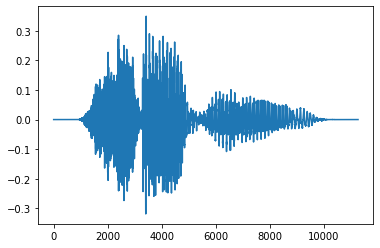
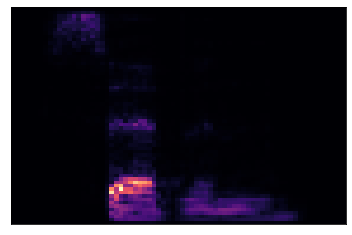
This is mostly what we do here, with one exception. Instead of applying the neural network directly on the input signal, first we make it more digestible while ensuring that all of the information that is important to the task is not lost. The transformation that is applied is called the Mel Spectrogram. It consists in computing the power of each frequency present in the sound on a scale that matches with typical human hearing abilities.
The deep learning model will then take this Mel Spectrogram as an input. But how can it convert this to text? One major difference between usual applications of neural networks (like distinguishing between pictures of cats and dogs) and Speech Recognition is that, in our case, the model has to return a sequence of variable length (the text) that might not be of length proportional to the length of the input. This problem is addressed with what is called the Connectionist Temporal Classification loss, or CTC loss. The main mechanism behind this loss is the operation of collapsing a given output sequence by combining every repeated character into one and then removing blank characters (shown as “_”).
"hhhheee__lll_ll___oooo____" gives "hello"
Basically, it allows the acoustic model to always return a matrix of length proportional to the sound duration, regardless of the number of characters that are needed. The output matrix contains the probability for each character in the alphabet (e.g. characters from “a” to “z” including the space and the blank character) at each time step (50 steps/sec in our case). Using this matrix, one can compute the probability of any voice command by summing the probabilities of all the sequences that can be collapsed to the command’s text.
The deep learning model that is able to convert the Mel Spectrogram into this CTC output can take various forms. In many cases it corresponds to a large and deep neural network that can contain hundreds of millions of parameters. This is likely to be out of reach for most mobile browsers on consumer devices. Thankfully, recent publications have proposed model architectures that can contain as few as 7 million parameters while maintaining a decent accuracy. In our case, we implemented the QuartzNet architecture proposed by a research team from Nvidia.
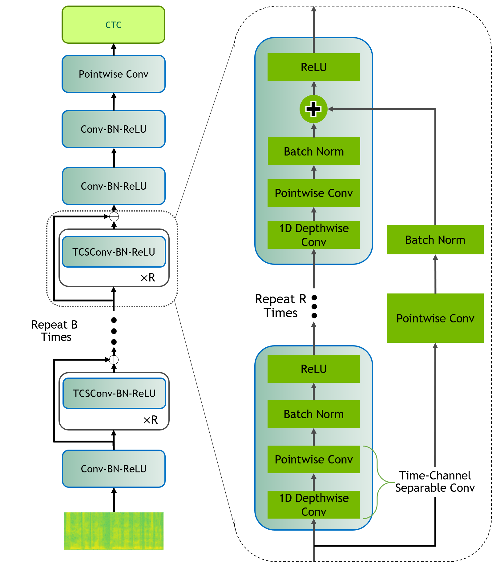
The QuartzNet architecture is based on the usage of separable convolutions while avoiding the use of any recurrent layer. Separable convolutions are neural network layers very similar to convolutions but have the advantage of requiring an order of magnitude fewer parameters. Also, the absence of any recurrent layer such as the LSTM layer enables the computation of the result to be done in a vastly more parallelizable way. The combination of these two choices makes for a model that is very light and fast to compute, which is exactly what we need.
Training infrastructure
Lastly, there is the problem of training this model. To do this, we started by collecting a few open datasets containing thousands of voice recordings along with their transcripts. We implemented the training module using TensorFlow as it is the natural choice to train a model that would later be loaded with TensorFlowJS. We built the input pipeline using the tf.data API as it enables us to avoid any bottleneck on the feature preprocessing side. It also makes it possible to stack multiple transformations made to the training data such as the data augmentations that we applied to make the model more robust to noise and to some variations in the input signal.
Then, we used the tf.estimator API for training as it provides many benefits. One of the most important benefit is that it fully manages the training and evaluation process of the model and requires no additional efforts to make it resilient to restarts. We will see why this is convenient in a few seconds. Also, the tf.estimator API makes it easy to export the model in a form that can contain the preprocessing with it, which is very handy as it removes the need to rewrite this functionality in JavaScript and further speeds up our ability to experiment with new ideas.
Now on the infrastructure part. We started by using training jobs on the GCP AI platform. This service provides a fully managed way to run your training module by automatically provisioning and deprovisioning VMs and keeping track of the resource usage and logs. This worked really well, however, there was an easy way to reduce costs significantly which would require us to move away from the AI platform. Along with regular VMs and the GPUs that can be attached to them, GCP also proposes preemptible VMs. They are identical to regular VMs and are about four times cheaper but they come with one tradeoff: they can be stopped at any moment. But as we have seen earlier, since our training module uses the tf.estimator API, it can easily pick up where it stopped as long as we always give it the same arguments. Knowing this, the only thing that we need is something that will have the ability to restart a new VM every time one is preempted. This can be straightforwardly achieved using GCP managed instance groups that can do exactly that. In the end, a simple 150 lines script was enough to launch a job using the gcloud command line interface. This is a very simple approach and it does not come with all the bells and whistles that tools like KubeFlow can provide, but it isc cheaper and much simpler to setup as it does not require a Kubernetes cluster that needs to run all the time.
The JavaScript library
Now that we have our acoustic model and after having converted it to a TensorFlowJS graph model, we need to write the code that will feed this model and compute the most probable commands being detected at each moment.
Overall architecture
In order to avoid excessive usage of the main thread, the library heavily relies on Web Workers. This way, the interface can stay fully responsive even while the recognition engine is running. Furthermore, continuously running the acoustic model on the input signal would not be wise as it would consume a large amount of processing power, therefore resulting in an excess use of the devices battery. To avoid this, we implemented an intermediate module to perform Voice Activity Detection.
The role of this module is to leverage a far simpler neural network model which only task is to detect when the input signal is likely to contain human speech. Given this information, we now have the ability to run the full acoustic model only when there might be some command being said. As this VAD module needs to run without interruption, we made it even more efficient by implementing it in C++ and compiling it to WebAssembly.
In addition to applying the deep learning model to the voice segments, the library finally needs to decode the raw output (the CTC matrix) into a structured object that can represent the spoken command. This last operation is quite important and deserves more explanations.
Decoding
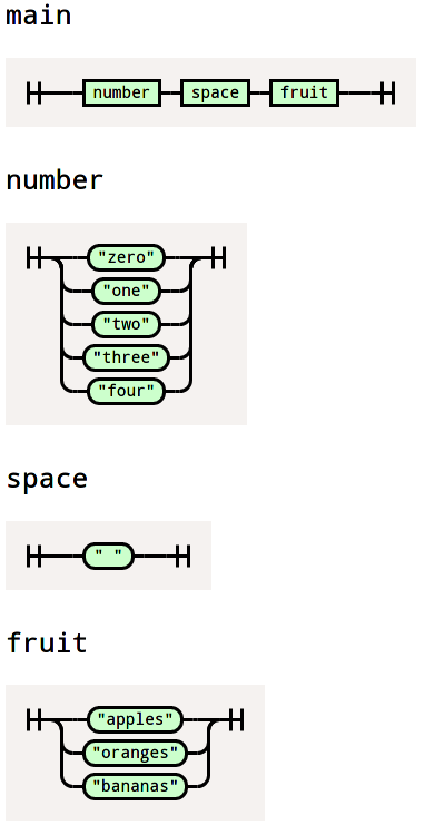
The way we specify the set of commands that are expected by the library is by providing a nearley grammar such as this one:
main -> number space fruit {% ([count, _, type]) => ({count, type}) %}

number -> "zero"   {% () => 0 %}
        | "one"    {% () => 1 %}
        | "two"    {% () => 2 %}
        | "three"  {% () => 3 %}
        | "four"   {% () => 4 %}

space -> " " {% () => null %}

fruit -> "apples"  {% () => "apple" %}
       | "oranges" {% () => "orange" %}
       | "bananas" {% () => "banana" %}
As you can see, a grammar enables us to define all the potential sequences that can be expected. It also has the added benefit of specifying how one should parse any given input in order to convert it to a structured object.
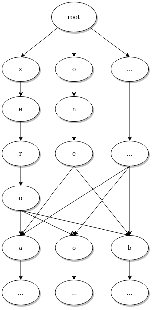
Once the output of the deep learning model has been computed, the usual beam search algorithm can then be applied. This algorithm looks for the most probable sequence of characters that respects the grammar. To do that, the grammar is first converted to a trie of individual characters, this data structure can be used to list every characters that are allowed after a given starting sequence.
The fact that the output sequences are constrained to respect the grammar has multiple advantages. The first one being that it is a lot quicker to compute since we don't have to consider every character at every time step. Also, it helps the acoustic model by acting as a bias towards the expected sequences. That is, even if the model "hesitates" between two words that might sound similar, the grammar will only accept the one that corresponds to a real spoken command if there is any. Finally, since the resulting text happens to respect the provided grammar, it can also be parsed by this same grammar in order to extract the detected command as a structured object.
"two apples" gives {count: 2, type: “apple”}
Overall usage
As described above, most of the heavy lifting is done inside Web Workers (VAD, model prediction, constrained beam search). The JavaScript library also makes sure that the model is downloaded once and then keeps it stored inside IndexedDB using native TFJS capabilities. All these characteristics make the library easy to use even on low end devices with poor internet connections.
As a user of this library, all I have to do is to specify the language to use, provide the grammar, and wait for commands to be sent to my callback as the combination of the command's text, the result after parsing and the associated probability. I can then use this result however appropriate to make the application react to it.
Conclusion
That’s it. Overall, we are quite happy with how simple the final project looks. There are many improvements that we hope to add in the future such as extending the use of WebAssembly to other parts of the library such as the acoustic model's inference. On the model aspect, in addition to running more experiments to make it even more accurate, it would also be interesting to make it even more space efficient by using sparse computations, which is not yet available in TFJS.
As this project was made from scratch, there can be many other things to discuss about it including our study about alternatives to TFJS, the reproducibility of the training jobs, or the various problems that we encountered with TensorFlow and TensorFlowJS. If you would like to see another article going deeper into any of these subjects including everything that was mentioned in this article, don’t hesitate to give feedback and tell us what you would want to see.
Paul Vanhaesebrouck – Data Scientist at Qima