Introduction
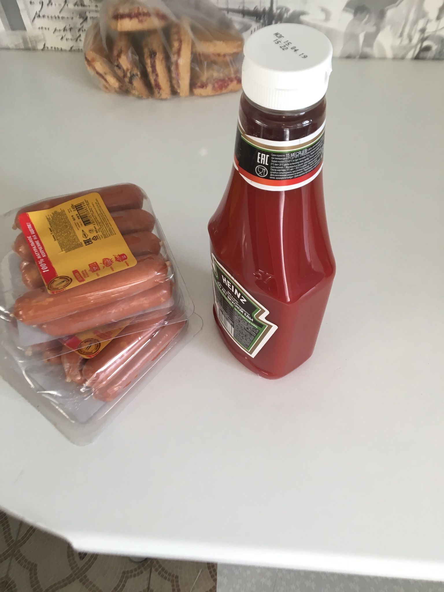
At QIMA, inspectors carry out inspections on all continents and deliver detailed reports on the various aspects of this process. These reports are full of photos, to illustrate various things (construction defects, product color...), which are taken in uncontrolled environments (luminosity, depth...) and with different cameras. Therefore, it is likely that defective photos will be taken, and it is essential to fix this by taking proper photos, as soon as possible in the process; to minimize risk that defective photos will have to be used in the final report.
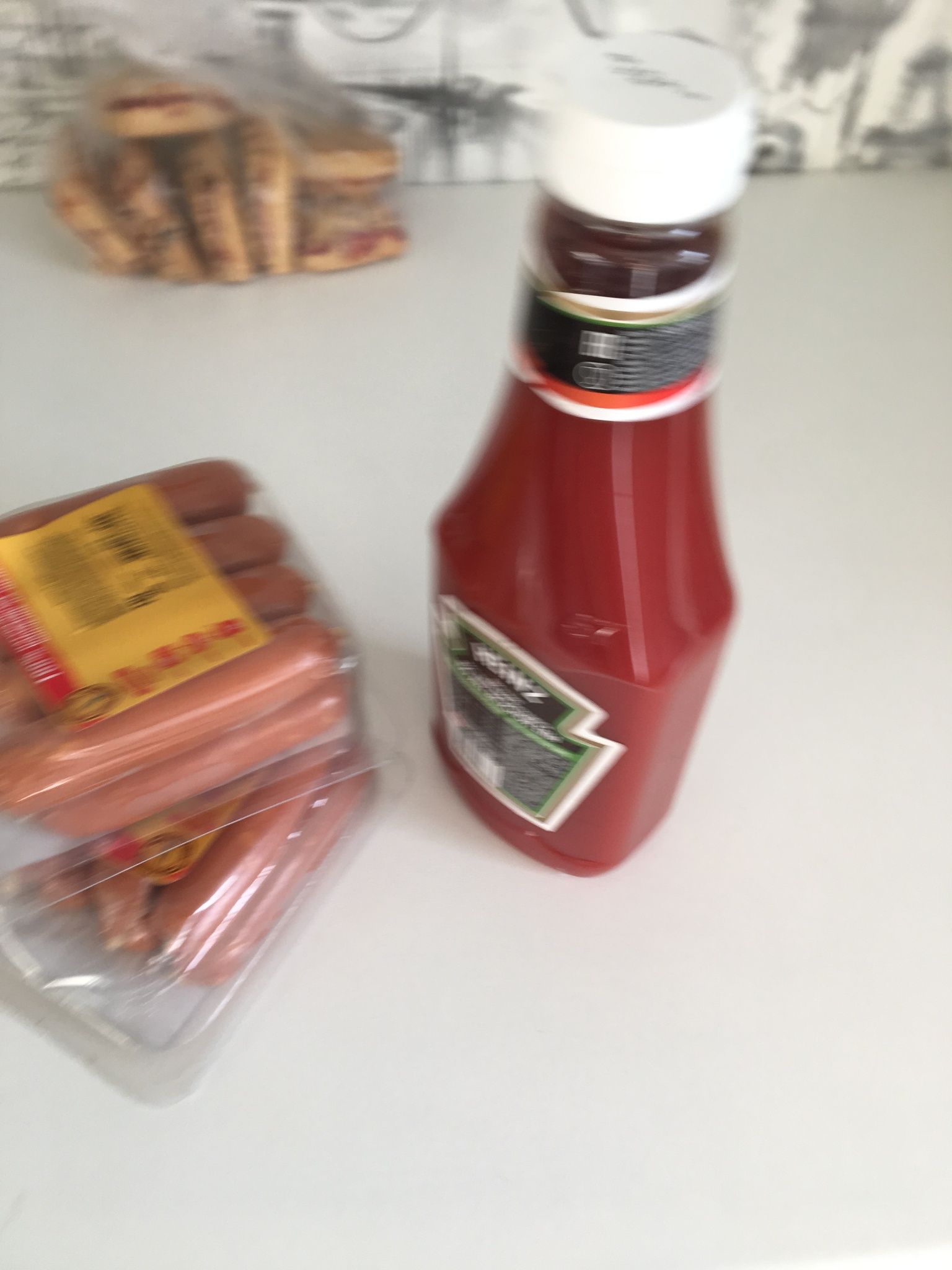
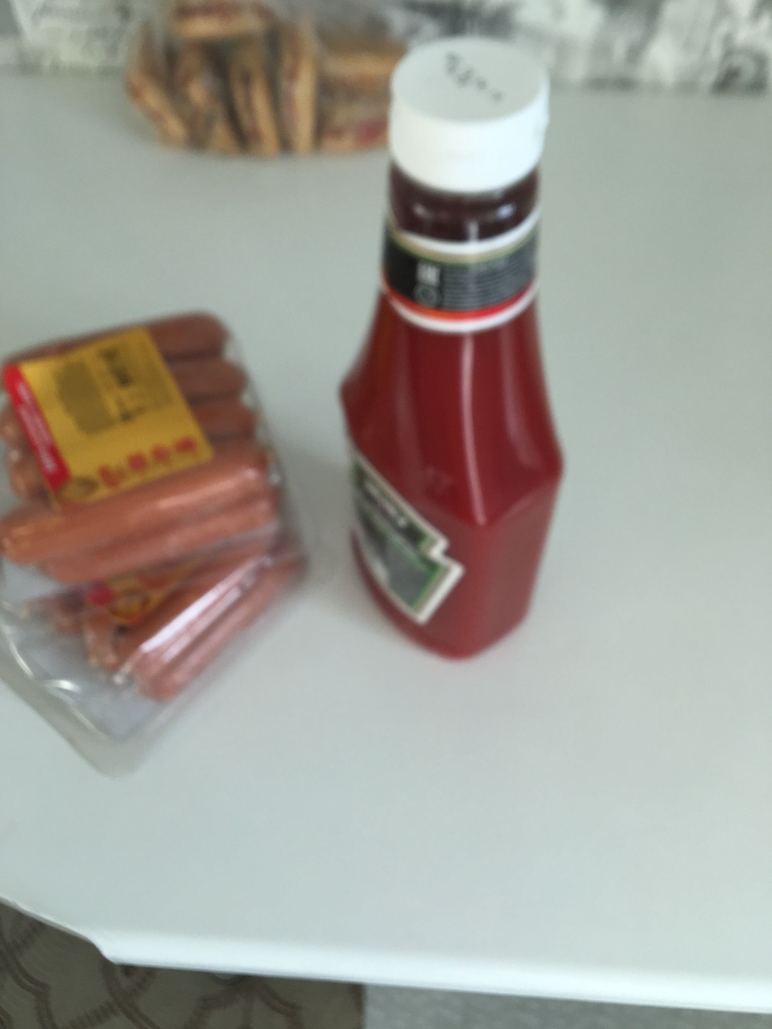
One of the main flaws that is recurrently found in the reports is that some photos are blurred.
Our goal was to create a model capable of identifying blurred photos and discerning what type of blur it is (motion, defocused). This way, the inspector knows what to do in order to re-take them correctly.
In this article we will show you how we have built a javascript library that allows our QIMAone web application to warn in real time the inspector each time a faulty photo is taken, and which works even without access to the internet.
Problem constraints
The main problem constraint is to train a model that is light enough to be integrated into the web application and used offline, as inspections can be conducted in very remote factories.
Dataset and preliminary work
For this problem, we wanted to distinguish three types of photos:
At first we wanted to see if we could tackle the problem with a relatively simple deep learning model using convolutional layers. But, when carrying out experiments, we faced issues with regards to the dataset: none really existed and were freely available that satisfied our needs. The one we ended up using at the time was that of someone who took various photos during their vacation, and then labelled them; whereas our uses cases are more about photos of products, taken from relatively close, and sometimes such that there is naturally not a lot of details in the photo. This lead to models with high false positive rates. Then, we tried to generate a proper dataset, by adding artificial blur to a set of sharp photos. However, the trained model was apparently able to recognize the artificial nature of the blur produced like that, and did not have a good enough level of generalization on photos were the blur was produced naturally. So we had to explore other possibilities.
Features engineering
By thinking about the properties of an image, and notably by using the sobel filter, we were able to craft two features that, when considered together, properly express all the relevant information needed to carry out this classification task.
Sobel filter
An image will be assumed to be a three dimensional tensor, whose dimensions are width, height, and depth, and whose values represent intensity. For a black and white image, there is only one layer of depth. For a color image, there can be three layer of depth, one for each of the following color channel: red, green, blue. In the following, we assume we are talking about a black and white image. As such, an image can be mathematically modeled as a one-dimension function over a discrete two-dimension input space.
To be able to analyze the images and distinguish which type of blur is present, we need to compute some quantities representing a certain type of information associated to the pixels of a given image:
- Magnitude, which indicates the intensity variation of an image around a given pixel
- Direction, which expresses the direction of growth of the intensity around a given pixel
This information can be calculated from the partial derivatives at each pixel of the image in the two directions x and y respectively.
A continuous partial derivative approximation in the x and y directions can be computed by convolving the image with appropriate kernels.
Here is an example of a convolution operation between an image representing a zebra and the kernel to obtain the partial derivatives along the y axis (the height of the image). On the picture, we can clearly see that the horizontal stripes of the zebra are highlighted compared to the vertical stripes.
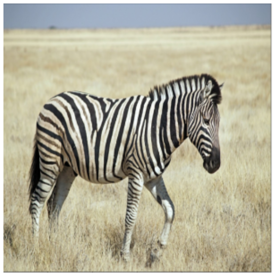
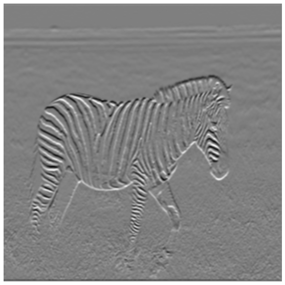
We would have had the opposite with the second kernel.
The kernels used are the following:
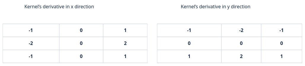
Those kernels are usually used to detect the edges of objects in an image. Indeed, it is around the edges that there is a rapid change in pixel intensity. However, it can also be used in our case, because when blur is present in an image, it will smooth the edges and the intensity will be reduced, especially for a defocused blur. For motion blur, it's a bit more subtle, as the presence of the smoothness depends on the direction in the image.
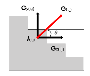
For a given pixel, once we have obtained the partial derivatives along the two axes, that we will note \(G_x\) and \(G_y\), we obtain the magnitude \(G\) and direction \( \Theta \) for each pixel as follows:
\[G = \sqrt{G_x^2 + G_y^2} \ \ \ \ \ \Theta = atan \left(\frac{G_y}{G_x} \right) \]
To have a geometrical representation of what we have just said, on the figure below, we have an image with 16 pixels representing the quarter of a full diamond. We can see the magnitude (which follows directly from the Pythagorean theorem) and its direction which is always orthogonal to the line of intensity change (i.e. the edge):
In the following section, we will assume that the image is square, and that the width size is equal to the height size, which is equal to n. One pixel will be identified by its row i and its column j, comprised between 0 and n-1.
First feature
The first feature is very simple and allows us to detect in particular the defocused blurs. Indeed, it is just a matter of taking the maximum value of magnitude for each image.
It is very likely that a sharp image will contain objects with well defined contours, and therefore high magnitudes while a defocused blurred image will have lower magnitudes as the intensity of each pixel will have been smoothed.
\[\underset{(i,j) \in [0; n-1]^{2}}{Max }\mathbf{G_{(i,j)}} \]
Regarding the motion blur, it is not as simple because the intensity of some pixels might be smoothed (i.e.: low magnitude) in a specific direction, but might be sharp / detailed (i.e.: high magnitude) in the orthogonal direction.
Second Feature
To be able to distinguish also motion blurs, we created a second feature that uses the direction of the intensity growth.
As we said before, motion blurred can smooth some pixels in one direction and can be sharp in the orthogonal direction. So we are looking for the clues of the existence of a direction such that the maximum magnitude along this direction is very low, whereas the maximum magnitude along the orthogonal direction is "normal", as can be expected in average in a sharp image.
Here is how we proceed: we split the first half of the trigonometric circle into B directions. For each direction, we will want to quantify whether the image contains details defined thanks to this direction, or if, on the contrary, the image is overall smooth in this direction. To do that, we group the pixels of the image into buckets associated to the different directions (using the direction of the gradient associated to a pixel, to determine in which bucket to place it), and we consider the maximum gradient magnitude value associated to the pixels found in a given bucket.
In this animation below, we can see an example of such a splitting of the trigonometric half circle, comprised between \( -\frac{\pi}{2} \) and \( \frac{\pi}{2} \). For example, below, the magnitude of the gradient (red arrow) will contribute to bucket n°8, because the direction of this gradient falls in the direction interval associated to that bucket.
To summarize what has been said, we obtain which pixel's magnitude belong to which bucket where we will take the maximum with the following formula:
\[ b_{(i,j)}= \sum_{s \in [-\pi /2,..., \pi /2]}[ G_y^{(i,j)} \times sign(G_x^{(i,j)}) \geq G_x^{(i,j)} \times \tan{s} \times sign(G_x^{(i,j)}) ] \]
Once we have the magnitude and the bucket corresponding to the intensity direction angle range for each pixel, we will take the maximum magnitude on each bucket:
\[ \forall b \in [0; B-1], G_{max^b} = \underset{(i,j) \in [0; n-1]^{2}}{Max} G^{b_{(i,j)}}\]
At the end, we get as many values as there are buckets.
Now comes the subtle part, it has been said that motion blur only smooths the change in intensity for a certain range of direction. In fact, when this happens, it is usually due to uncontrolled camera movement during the shooting process. This movement usually follows one direction in space. So one can expect to have a lower magnitude for a given bucket corresponding to a direction range.
To distinguish this, we will take the cosine and sine for angle values between 0 and \(2\pi \), divided by the number of buckets. We will obtain our second feature with the following formula:
\[ \sqrt{ (G^T_{max}.cos^b)^2 + (G^T_{max}.sin^b)^2}\]
with \(cos^b = [cos \left( \frac{i*2\pi}{B} \right)] \) and \(sin^b = [sin \left( \frac{i*2\pi}{B} \right)] \) and \( G^T_{max} = [ G_{max}^i ], \ \forall i \in [0; B - 1] \)
Let's say we have a defocused blurred image, the intensity changes corresponding to the contours of objects are smoothed. Whatever the direction of intensity growth, the magnitude is likely to be low. Now let's take a sharp image, with well defined objects. The magnitude is likely to be strong in any direction. (Exception if the image in question is monochrome, with few edges).
For the sake of simplicity, for both cases, we can assume that the magnitude value for each bucket is constant. The above formula then becomes:
\[ G^T_{max} \times \sqrt{ (\sum_{i=0}^{B-1} cos( \frac{i*2\pi}{B}))^2 + (\sum_{i=0}^{B-1} sin ( \frac{i*2\pi}{B}))^2} \]
with
\[ \sum_{i=0}^{B-1} cos( \frac{i*2\pi}{B}) = 0 + \epsilon \ and \ \sum_{i=0}^{B-1} sin( \frac{i*2\pi}{B}) = 0 + \epsilon \]
with epsilon the noise due to the fact that we took discrete values in the interval [0,2π]. We would have obtained 0 if the number of buckets tended towards infinity. Even if this had been the case, it is very unlikely to reach 0 because we have made a strong assumption about the value of the magnitudes being constant over each bucket. These quantities remain close to 0.
Now take an image with motion blur, and assume that the magnitude is very high in one particular bucket, corresponding to the bucket of the orthogonal direction of motion blur present in the image and very low in an another one, corresponding to the bucket of the direction of motion blur present in the image. The difference in magnitude between buckets will be captured by the sine or cosine.
To better understand, here are two animations (Click on it to see the details) :
- Sharp image
- Image with motion blur
Model and Training
We have chosen as model the logistic regression, which is a machine learning algorithm very widespread in the resolution of classification problems. We will not dwell on the mathematics behind this model, nor explain how it works, there are many good resources on this subject such as here.
To train the model, we started by manually creating our labelled data. We then implemented the training module using TensorFlow as we would like to convert it to TensorflowJS graph model which will allow us to use the model directly on the web application.
To convert the model easily, we used the Keras library which uses Tensorflow back-end by default. To obtain the logistic regression model using a deep learning library, we used a neural network with no hidden layer and a layer with one neuron. By using the softmax activation function, we obtained the logistic regression model. In the image below, we have an example of the architecture of the model with 3 inputs:
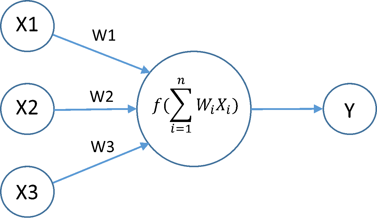 with f the softmax activation function.
The JavaScript library
Now that we have our model and after having converted it to a TensorFlowJS graph model, we need to write the code that will feed this model and compute the result for each image that has been taken by inspectors.
During the inspection, this library will provide images to the model and will display appropriate messages for each scenario, such as: "Try not to move your phone when you take the picture" if it is one with motion blur.
After using the machine learning model, it will process the obtained probabilities as follows:
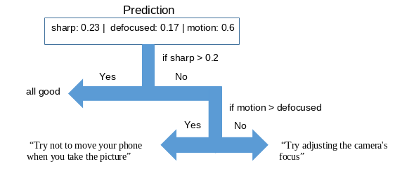
Inspectors will have the choice to keep or remove photos designated as blurred by the application model.
Conclusion
Technically, we are satisfied with the model and the features are quite interesting (especially the second one). However, there are still rooms for improvement, notably the implementation of a pipeline that would allow us to retrieve the blurred photos kept by the inspectors on the application in order to create more stable models. We can also adjust features as well as improve the model.
We are hiring a Senior Data Scientist ;) https://www.welcometothejungle.com/fr/companies/qima/jobs/data-scientist-senior_paris
Sadi-Cherif Abdulaziz – Data Scientist at QIMA